Resilient Distributed Datasets:
A Fault-Tolerant Abstraction for In-Memory Cluster Computing
Matei Zaharia, Mosharaf Chowdhury, Tathagata Das, Ankur Dave, Justin Ma, Murphy McCauley, Michael J. Franklin, Scott Shenker, Ion Stoica
University of California, Berkeley
Abstract (초록)
We present Resilient Distributed Datasets (RDDs), a distributed memory abstraction that lets programmers perform in-memory computations on large clusters in a fault-tolerant manner. RDDs are motivated by two types of applications that current computing frameworks handle inefficiently: iterative algorithms and interactive data mining tools. In both cases, keeping data in memory can improve performance by an order of magnitude.
우리는 Resilient Distributed Datasets(RDDs)을 소개한다. 이는 대규모 클러스터에서 메모리 내 연산을 장애 복구가 가능한 방식으로 수행할 수 있도록 해주는 분산 메모리 추상화이다. RDDs는 현재의 컴퓨팅 프레임워크가 비효율적으로 처리하는 두 가지 유형의 애플리케이션에서 동기부여를 받았다: 반복적 알고리즘과 대화형 데이터 마이닝 도구. 이 두 경우에서 데이터를 메모리에 유지하면 성능이 한 자리 수 이상 향상될 수 있다.
To achieve fault tolerance efficiently, RDDs provide a restricted form of shared memory, based on coarsegrained transformations rather than fine-grained updates to shared state. However, we show that RDDs are expressive enough to capture a wide class of computations, including recent specialized programming models for iterative jobs, such as Pregel, and new applications that these models do not capture. We have implemented RDDs in a system called Spark, which we evaluate through a variety of user applications and benchmarks.
장애 복구를 효율적으로 달성하기 위해, RDDs는 미세한 상태 업데이트가 아닌, 거친 변환을 기반으로 하는 제한된 형태의 공유 메모리를 제공한다. 그러나 우리는 RDDs가 Pregel과 같은 반복적 작업을 위한 최신 특수 프로그래밍 모델뿐만 아니라, 이러한 모델이 포착하지 못하는 새로운 애플리케이션까지 포함할 수 있을 만큼 충분히 표현력이 풍부하다는 것을 보여준다.
우리는 RDDs를 Spark라는 시스템으로 구현하였으며, 이를 다양한 사용자 애플리케이션과 벤치마크를 통해 평가하였다.
1 Introduction
Cluster computing frameworks like MapReduce [10] and Dryad [19] have been widely adopted for large-scale data analytics. These systems let users write parallel computations using a set of high-level operators, without having to worry about work distribution and fault tolerance.
MapReduce [10] 및 Dryad [19]와 같은 클러스터 컴퓨팅 프레임워크는 대규모 데이터 분석을 위해 널리 채택되었다. 이러한 시스템은 사용자가 작업 분배와 장애 복구를 걱정할 필요 없이, 고수준 연산자의 집합을 사용하여 병렬 연산을 작성할 수 있도록 해준다.
Although current frameworks provide numerous abstractions for accessing a cluster’s computational resources, they lack abstractions for leveraging distributed memory. This makes them inefficient for an important class of emerging applications: those that reuse intermediate results across multiple computations. Data reuse is common in many iterative machine learning and graph algorithms, including PageRank, K-means clustering, and logistic regression. Another compelling use case is interactive data mining, where a user runs multiple adhoc queries on the same subset of the data.
현재의 프레임워크는 클러스터의 계산 자원에 접근하기 위한 다양한 추상화를 제공하지만, 분산 메모리를 활용하기 위한 추상화는 부족하다. 이로 인해, 여러 계산에서 중간 결과를 재사용하는 애플리케이션과 같은 중요한 새로운 유형의 애플리케이션에 대해 비효율적이다. 데이터 재사용은 PageRank, K-means 클러스터링, 로지스틱 회귀와 같은 많은 반복적 기계 학습 및 그래프 알고리즘에서 일반적으로 발생한다. 또 다른 중요한 사례는 대화형 데이터 마이닝으로, 사용자가 동일한 데이터 하위 집합에 대해 여러 개의 즉석 질의를 실행하는 경우이다.
Unfortunately, in most current frameworks, the only way to reuse data between computations (e.g., between two MapReduce jobs) is to write it to an external stable storage system, e.g., a distributed file system. This incurs substantial overheads due to data replication, disk I/O, and serialization, which can dominate application execution times.
안타깝게도, 대부분의 기존 프레임워크에서는 연산 간(예: 두 개의 MapReduce 작업 간) 데이터를 재사용하는 유일한 방법이 데이터를 외부의 안정적인 저장소 시스템, 예를 들어 분산 파일 시스템에 기록하는 것이다. 이는 데이터 복제, 디스크 I/O, 직렬화로 인해 상당한 오버헤드를 초래하며, 이는 애플리케이션 실행 시간을 지배할 수 있다.
Recognizing this problem, researchers have developed specialized frameworks for some applications that require data reuse. For example, Pregel [22] is a system for iterative graph computations that keeps intermediate data in memory, while HaLoop [7] offers an iterative MapReduce interface. However, these frameworks only support specific computation patterns (e.g., looping a series of MapReduce steps), and perform data sharing implicitly for these patterns. They do not provide abstractions for more general reuse, e.g., to let a user load several datasets into memory and run ad-hoc queries across them.
이 문제를 인식한 연구자들은 데이터 재사용이 필요한 일부 애플리케이션을 위해 특수한 프레임워크를 개발해왔다. 예를 들어, Pregel [22]은 중간 데이터를 메모리에 유지하는 반복적 그래프 연산을 위한 시스템이며, HaLoop [7]은 반복적 MapReduce 인터페이스를 제공한다. 그러나 이러한 프레임워크는 특정한 연산 패턴(예: 일련의 MapReduce 단계를 반복하는 것)만을 지원하며, 이러한 패턴에 대해 암묵적으로 데이터 공유를 수행한다. 이들은 보다 일반적인 데이터 재사용을 위한 추상화를 제공하지 않으며, 예를 들어 사용자가 여러 개의 데이터셋을 메모리에 로드한 후 즉석 질의를 실행하는 것을 지원하지 않는다.
In this paper, we propose a new abstraction called resilient distributed datasets (RDDs) that enables efficient data reuse in a broad range of applications. RDDs are fault-tolerant, parallel data structures that let users explicitly persist intermediate results in memory, control their partitioning to optimize data placement, and manipulate them using a rich set of operators.
이 논문에서는 다양한 애플리케이션에서 효율적인 데이터 재사용을 가능하게 하는 resilient distributed datasets (RDDs)라는 새로운 추상화를 제안한다. RDDs는 장애 복구가 가능하며 병렬 처리를 지원하는 데이터 구조로, 사용자가 중간 결과를 명시적으로 메모리에 유지하고, 데이터 배치를 최적화하기 위해 파티셔닝을 제어하며, 다양한 연산자를 사용하여 데이터를 조작할 수 있도록 한다.
The main challenge in designing RDDs is defining a programming interface that can provide fault tolerance efficiently. Existing abstractions for in-memory storage on clusters, such as distributed shared memory [24], keyvalue stores [25], databases, and Piccolo [27], offer an interface based on fine-grained updates to mutable state (e.g., cells in a table). With this interface, the only ways to provide fault tolerance are to replicate the data across machines or to log updates across machines. Both approaches are expensive for data-intensive workloads, as they require copying large amounts of data over the cluster network, whose bandwidth is far lower than that of RAM, and they incur substantial storage overhead.
RDD를 설계하는 데 있어 주요 과제는 장애 복구를 효율적으로 제공할 수 있는 프로그래밍 인터페이스를 정의하는 것이다. 분산 공유 메모리, 키-값 저장소, 데이터베이스, Piccolo [27]와 같은 기존의 클러스터 내 메모리 저장소를 위한 추상화는 가변 상태의 미세한 업데이트(예: 테이블의 개별 셀)를 기반으로 하는 인터페이스를 제공한다. 이러한 인터페이스에서는 장애 복구를 제공하는 유일한 방법이 데이터를 여러 머신에 복제하거나, 업데이트를 여러 머신에 기록하는 것이다. 그러나 두 방식 모두 데이터 집약적인 작업에 있어 비용이 많이 든다. 이는 클러스터 네트워크의 대역폭이 RAM보다 훨씬 낮기 때문에 대량의 데이터를 네트워크를 통해 복사해야 하며, 상당한 저장 오버헤드를 초래하기 때문이다.
In contrast to these systems, RDDs provide an interface based on coarse-grained transformations (e.g., map, filter and join) that apply the same operation to many data items. This allows them to efficiently provide fault tolerance by logging the transformations used to build a dataset (its lineage) rather than the actual data.* If a partition of an RDD is lost, the RDD has enough information about how it was derived from other RDDs to recompute just that partition. Thus, lost data can be recovered, often quite quickly, without requiring costly replication.
* Checkpointing the data in some RDDs may be useful when a lineage chain grows large, however, and we discuss how to do it in §5.4
이러한 시스템들과 달리, RDDs는 여러 데이터 항목에 동일한 연산을 적용하는 거친 단위의 변환(map, filter, join 등)을 기반으로 하는 인터페이스를 제공한다. 이를 통해, 실제 데이터를 기록하는 대신 데이터셋을 생성하는 데 사용된 변환 과정(계보)을 기록함으로써 효율적으로 장애 복구를 제공할 수 있다. * RDD의 특정 파티션이 손실되면, RDD는 다른 RDD들로부터 해당 파티션이 어떻게 생성되었는지에 대한 충분한 정보를 가지고 있어, 해당 파티션만 다시 계산할 수 있다. 따라서 손실된 데이터를 비용이 많이 드는 복제 없이도, 종종 매우 빠르게 복구할 수 있다.
* 일부 RDD에서 계보 체인이 너무 길어질 경우 데이터를 체크포인트하는 것이 유용할 수 있으며, 이에 대한 방법을 §5.4에서 논의한다.
Although an interface based on coarse-grained transformations may at first seem limited, RDDs are a good fit for many parallel applications, because these applications naturally apply the same operation to multiple data items. Indeed, we show that RDDs can efficiently express many cluster programming models that have so far been proposed as separate systems, including MapReduce, DryadLINQ, SQL, Pregel and HaLoop, as well as new applications that these systems do not capture, like interactive data mining. The ability of RDDs to accommodate computing needs that were previously met only by introducing new frameworks is, we believe, the most credible evidence of the power of the RDD abstraction.
거친 단위의 변환을 기반으로 한 인터페이스는 처음에는 제한적으로 보일 수 있지만, RDDs는 많은 병렬 애플리케이션에 적합하다. 이는 이러한 애플리케이션이 본질적으로 여러 데이터 항목에 동일한 연산을 적용하기 때문이다. 실제로 우리는 RDDs가 기존에 개별 시스템으로 제안되었던 다양한 클러스터 프로그래밍 모델을 효율적으로 표현할 수 있음을 보여준다. 여기에는 MapReduce, DryadLINQ, SQL, Pregel, HaLoop뿐만 아니라, 기존 시스템이 포착하지 못하는 대화형 데이터 마이닝과 같은 새로운 애플리케이션도 포함된다. 이전에는 새로운 프레임워크를 도입해야만 가능했던 컴퓨팅 요구를 RDDs가 수용할 수 있다는 점이야말로, RDD 추상화의 강력함을 입증하는 가장 신뢰할 만한 증거라고 생각한다.
We have implemented RDDs in a system called Spark, which is being used for research and production applications at UC Berkeley and several companies. Spark provides a convenient language-integrated programming interface similar to DryadLINQ [31] in the Scala programming language [2]. In addition, Spark can be used interactively to query big datasets from the Scala interpreter. We believe that Spark is the first system that allows a general-purpose programming language to be used at interactive speeds for in-memory data mining on clusters.
우리는 RDDs를 Spark라는 시스템으로 구현하였으며, 이는 UC Berkeley와 여러 기업에서 연구 및 실무 애플리케이션에 활용되고 있다. Spark는 Scala 프로그래밍 언어에서 DryadLINQ와 유사한 편리한 언어 통합 프로그래밍 인터페이스를 제공한다. 또한, Spark는 Scala 인터프리터에서 대규모 데이터셋을 대화형으로 질의하는 데 사용할 수 있다. 우리는 Spark가 클러스터에서 메모리 내 데이터 마이닝을 대화형 속도로 수행할 수 있도록 범용 프로그래밍 언어를 지원하는 최초의 시스템이라고 생각한다.
We evaluate RDDs and Spark through both microbenchmarks and measurements of user applications. We show that Spark is up to 20× faster than Hadoop for iterative applications, speeds up a real-world data analytics report by 40×, and can be used interactively to scan a 1 TB dataset with 5–7s latency. More fundamentally, to illustrate the generality of RDDs, we have implemented the Pregel and HaLoop programming models on top of Spark, including the placement optimizations they employ, as relatively small libraries (200 lines of code each).
우리는 RDDs와 Spark를 마이크로벤치마크와 사용자 애플리케이션 측정을 통해 평가한다. 우리는 Spark가 반복적 애플리케이션에서 Hadoop보다 최대 20배 빠르며, 실제 데이터 분석 보고서를 40배 빠르게 처리하고, 1TB 데이터셋을 5~7초의 지연 시간으로 대화형으로 스캔하는 데 사용할 수 있음을 보여준다. 더욱 근본적으로, RDDs의 범용성을 입증하기 위해, 우리는 Pregel 및 HaLoop 프로그래밍 모델을 Spark 위에 구현하였으며, 이들이 사용하는 데이터 배치 최적화 기법을 포함하더라도 각각 약 200줄의 비교적 작은 라이브러리로 작성할 수 있음을 보였다.
This paper begins with an overview of RDDs (§2) and Spark (§3). We then discuss the internal representation of RDDs (§4), our implementation (§5), and experimental results (§6). Finally, we discuss how RDDs capture several existing cluster programming models (§7), survey related work (§8), and conclude.
이 논문은 RDDs 개요(§2)와 Spark 개요(§3)로 시작한다. 이후, RDDs의 내부 표현 방식(§4), 우리의 구현(§5), 실험 결과(§6)를 논의한다. 마지막으로, RDDs가 기존의 여러 클러스터 프로그래밍 모델을 어떻게 포착하는지 설명(§7)하고, 관련 연구를 검토(§8)한 후 결론을 맺는다.
2 Resilient Distributed Datasets (RDDs)
This section provides an overview of RDDs. We first define RDDs (§2.1) and introduce their programming interface in Spark (§2.2). We then compare RDDs with finergrained shared memory abstractions (§2.3). Finally, we discuss limitations of the RDD model (§2.4).
이 섹션에서는 RDDs에 대한 개요를 제공한다. 먼저, RDDs를 정의하고(§2.1), Spark에서의 프로그래밍 인터페이스를 소개한다(§2.2). 이후, RDDs를 보다 세밀한 공유 메모리 추상화와 비교한다(§2.3). 마지막으로, RDD 모델의 한계점에 대해 논의한다(§2.4).
2.1 RDD Abstraction
Formally, an RDD is a read-only, partitioned collection of records. RDDs can only be created through deterministic operations on either (1) data in stable storage or (2) other RDDs. We call these operations transformations to differentiate them from other operations on RDDs. Examples of transformations include map, filter, and join. *
형식적으로, RDD는 읽기 전용이며 파티션된 레코드의 집합이다. RDD는 오직 (1) 안정적인 저장소에 있는 데이터 또는 (2) 다른 RDD에 대해 결정론적 연산을 수행함으로써 생성될 수 있다. 이러한 연산을 RDD의 다른 연산들과 구별하기 위해 변환(transformations)이라고 부른다. 변환의 예로는 map, filter, join 등이 있다.
* Although individual RDDs are immutable, it is possible to implement mutable state by having multiple RDDs to represent multiple versions of a dataset. We made RDDs immutable to make it easier to describe lineage graphs, but it would have been equivalent to have our abstraction be versioned datasets and track versions in lineage graphs.
* 개별 RDD는 변경할 수 없지만, 여러 RDD를 사용하여 데이터셋의 여러 버전을 표현함으로써 가변 상태를 구현하는 것은 가능하다. 우리는 계보 그래프를 더 쉽게 설명할 수 있도록 RDD를 불변하도록 만들었지만, 버전이 있는 데이터셋을 추상화하고 계보 그래프에서 버전을 추적하는 방식과 본질적으로 동일한 결과를 얻을 수 있다.
RDDs do not need to be materialized at all times. Instead, an RDD has enough information about how it was derived from other datasets (its lineage) to compute its partitions from data in stable storage. This is a powerful property: in essence, a program cannot reference an RDD that it cannot reconstruct after a failure.
RDD는 항상 실체화될 필요가 없다. 대신, RDD는 안정적인 저장소에 있는 데이터로부터 자신의 파티션을 계산할 수 있도록, 다른 데이터셋으로부터 어떻게 유도되었는지에 대한 충분한 정보(계보)를 가지고 있다. 이는 강력한 속성으로, 본질적으로 프로그램은 장애 발생 후 복구할 수 없는 RDD를 참조할 수 없다.
Finally, users can control two other aspects of RDDs: persistence and partitioning. Users can indicate which RDDs they will reuse and choose a storage strategy for them (e.g., in-memory storage). They can also ask that an RDD’s elements be partitioned across machines based on a key in each record. This is useful for placement optimizations, such as ensuring that two datasets that will be joined together are hash-partitioned in the same way.
마지막으로, 사용자는 RDD의 두 가지 측면인 지속성과 파티셔닝을 제어할 수 있다. 사용자는 어떤 RDD를 재사용할 것인지 지정하고, 해당 RDD의 저장 전략(예: 메모리 내 저장)을 선택할 수 있다. 또한, 각 레코드의 키를 기반으로 RDD의 요소가 여러 머신에 걸쳐 파티셔닝되도록 요청할 수도 있다. 이는 두 개의 데이터셋을 동일한 방식으로 해시 파티셔닝하여 조인의 성능을 최적화하는 등 데이터 배치를 효율적으로 조정하는 데 유용하다.
2.2 Spark Programming Interface
Spark exposes RDDs through a language-integrated API similar to DryadLINQ [31] and FlumeJava [8], where each dataset is represented as an object and transformations are invoked using methods on these objects.
Spark는 RDD를 DryadLINQ [31] 및 FlumeJava [8]와 유사한 언어 통합 API를 통해 제공하며, 각 데이터셋은 객체로 표현되고 변환은 이러한 객체의 메서드를 통해 호출된다.
Programmers start by defining one or more RDDs through transformations on data in stable storage (e.g., map and filter). They can then use these RDDs in actions, which are operations that return a value to the application or export data to a storage system. Examples of actions include count (which returns the number of elements in the dataset), collect (which returns the elements themselves), and save (which outputs the dataset to a storage system). Like DryadLINQ, Spark computes RDDs lazily the first time they are used in an action, so that it can pipeline transformations.
프로그래머는 안정적인 저장소의 데이터에 대한 변환(e.g., map and filter)을 통해 하나 이상의 RDD를 정의하는 것부터 시작한다. 이후, 이러한 RDD를 애플리케이션에 값을 반환하거나 데이터를 저장소 시스템에 내보내는 작업인 액션에서 사용할 수 있다. 액션의 예로는 count(데이터셋의 요소 개수를 반환), collect(요소 자체를 반환), save(데이터셋을 저장소 시스템에 출력) 등이 있다. DryadLINQ와 마찬가지로, Spark는 RDD가 액션에서 처음 사용될 때 지연 계산(lazily)을 수행하여 변환을 파이프라이닝할 수 있도록 한다.
In addition, programmers can call a persist method to indicate which RDDs they want to reuse in future operations. Spark keeps persistent RDDs in memory by default, but it can spill them to disk if there is not enough RAM. Users can also request other persistence strategies, such as storing the RDD only on disk or replicating it across machines, through flags to persist. Finally, users can set a persistence priority on each RDD to specify which in-memory data should spill to disk first.
또한, 프로그래머는 persist 메서드를 호출하여 향후 연산에서 재사용할 RDD를 지정할 수 있다. Spark는 기본적으로 지속적인 RDD를 메모리에 유지하지만, RAM이 부족할 경우 디스크로 내보낼 수 있다. 사용자는 persist에 전달하는 플래그를 통해 RDD를 디스크에만 저장하거나 여러 머신에 복제하는 등 다른 지속성 전략을 요청할 수도 있다. 마지막으로, 사용자는 각 RDD에 대해 지속성 우선순위를 설정하여 어떤 메모리 내 데이터가 먼저 디스크로 내보내질지를 지정할 수 있다.
2.2.1 Example: Console Log Mining
Suppose that a web service is experiencing errors and an operator wants to search terabytes of logs in the Hadoop filesystem (HDFS) to find the cause. Using Spark, the operator can load just the error messages from the logs into RAM across a set of nodes and query them interactively. She would first type the following Scala code:
예를 들어, 웹 서비스에서 오류가 발생하고 있으며 운영자가 Hadoop 파일 시스템(HDFS)에 저장된 테라바이트 규모의 로그를 검색하여 원인을 찾고자 한다고 가정하자. Spark를 사용하면 운영자는 로그에서 오류 메시지만을 선택하여 여러 노드의 RAM에 로드하고, 이를 대화형으로 질의할 수 있다. 먼저, 운영자는 다음과 같은 Scala 코드를 입력할 것이다.

lines = spark.textFile("hdfs://...")
errors = lines.filter(_.startsWith("ERROR"))
errors.persist()
Line 1 defines an RDD backed by an HDFS file (as a collection of lines of text), while line 2 derives a filtered RDD from it. Line 3 then asks for errors to persist in memory so that it can be shared across queries. Note that the argument to filter is Scala syntax for a closure.
1행은 HDFS 파일을 기반으로 하는 RDD를 정의하며, 이는 텍스트 줄의 집합으로 구성된다. 2행에서는 해당 RDD에서 필터링된 RDD를 생성한다. 3행에서는 오류 메시지가 메모리에 유지되도록 persist를 호출하여, 이후의 질의에서 공유될 수 있도록 한다. 필터 함수의 인자가 클로저를 표현하는 Scala 문법이라는 점에 주목해야 한다.
At this point, no work has been performed on the cluster. However, the user can now use the RDD in actions, e.g., to count the number of messages:
이 시점에서는 클러스터에서 아직 어떤 연산도 수행되지 않았다. 그러나 이제 사용자는 RDD를 액션에서 사용할 수 있으며, 예를 들어 메시지의 개수를 세는 작업을 수행할 수 있다.
errors.count()
The user can also perform further transformations on the RDD and use their results, as in the following lines:
사용자는 또한 RDD에 대해 추가적인 변환을 수행하고, 그 결과를 활용할 수도 있다. 다음 코드와 같이 사용할 수 있다.
// "MySQL"을 언급하는 오류의 개수를 계산
errors.filter(_.contains("MySQL")).count()
// "HDFS"를 언급하는 오류의 시간 필드를 배열로 반환
// (시간 필드가 탭으로 구분된 형식에서 세 번째 필드라고 가정)
errors.filter(_.contains("HDFS"))
.map(_.split('\t')(3))
.collect()
After the first action involving errors runs, Spark will store the partitions of errors in memory, greatly speeding up subsequent computations on it. Note that the base RDD, lines, is not loaded into RAM. This is desirable because the error messages might only be a small fraction of the data (small enough to fit into memory).
errors RDD를 사용하는 첫 번째 액션이 실행된 후, Spark는 errors의 파티션을 메모리에 저장하여 이후의 연산을 크게 가속화한다. 하지만 기본 RDD인 lines는 RAM에 로드되지 않는다. 이는 오류 메시지가 전체 데이터의 작은 일부에 불과할 가능성이 높으며, 메모리에 충분히 저장될 수 있기 때문에 바람직한 동작이다.
Finally, to illustrate how our model achieves fault tolerance, we show the lineage graph for the RDDs in our third query in Figure 1. In this query, we started with errors, the result of a filter on lines, and applied a further filter and map before running a collect. The Spark scheduler will pipeline the latter two transformations and send a set of tasks to compute them to the nodes holding the cached partitions of errors. In addition, if a partition of errors is lost, Spark rebuilds it by applying a filter on only the corresponding partition of lines.
마지막으로, 우리의 모델이 어떻게 장애 복구를 달성하는지 설명하기 위해, 세 번째 질의에서 사용된 RDD들의 계보 그래프를 그림 1에 나타낸다. 이 질의에서는 lines에 대한 filter 연산의 결과인 errors에서 시작하여, 추가적인 filter와 map을 적용한 후 collect를 실행했다. Spark 스케줄러는 후자의 두 변환을 파이프라이닝하여, errors의 캐시된 파티션을 보유한 노드에서 이를 계산하는 작업들을 전송한다. 또한, errors의 특정 파티션이 손실되면, Spark는 해당 파티션과 연관된 lines의 파티션에 filter를 적용하여 이를 재구성한다.

2.3 Advantages of the RDD Model
To understand the benefits of RDDs as a distributed memory abstraction, we compare them against distributed shared memory (DSM) in Table 1. In DSM systems, applications read and write to arbitrary locations in a global address space. Note that under this definition, we include not only traditional shared memory systems [24], but also other systems where applications make finegrained writes to shared state, including Piccolo [27], which provides a shared DHT, and distributed databases. DSM is a very general abstraction, but this generality makes it harder to implement in an efficient and faulttolerant manner on commodity clusters.
RDD가 분산 메모리 추상화로서 가지는 이점을 이해하기 위해, 표 1에서 분산 공유 메모리(DSM)와 비교한다. DSM 시스템에서는 애플리케이션이 전역 주소 공간의 임의의 위치에서 데이터를 읽고 쓸 수 있다. 이러한 정의에 따르면, 기존의 공유 메모리 시스템 [24]뿐만 아니라, 공유 DHT를 제공하는 Piccolo [27] 및 분산 데이터베이스와 같이 애플리케이션이 공유 상태에 대해 세밀한 단위의 쓰기를 수행하는 다른 시스템들도 포함된다. DSM은 매우 일반적인 추상화이지만, 이러한 일반성이 상용 클러스터에서 효율적이고 장애 복구가 가능한 방식으로 구현되는 것을 어렵게 만든다.
The main difference between RDDs and DSM is that RDDs can only be created (“written”) through coarsegrained transformations, while DSM allows reads and writes to each memory location.3 This restricts RDDs to applications that perform bulk writes, but allows for more efficient fault tolerance. In particular, RDDs do not need to incur the overhead of checkpointing, as they can be recovered using lineage.4 Furthermore, only the lost partitions of an RDD need to be recomputed upon failure, and they can be recomputed in parallel on different nodes, without having to roll back the whole program.
RDD와 DSM의 가장 큰 차이점은 RDD는 거친 단위의 변환을 통해서만 생성(“쓰기”)될 수 있는 반면, DSM은 각 메모리 위치에 대한 읽기 및 쓰기가 가능하다는 점이다. 이러한 제한으로 인해 RDD는 대량 쓰기 작업을 수행하는 애플리케이션에만 적합하지만, 훨씬 더 효율적인 장애 복구가 가능하다. 특히, RDD는 계보(lineage)를 활용하여 복구할 수 있기 때문에 체크포인트 작업의 오버헤드를 발생시킬 필요가 없다. 또한, 장애 발생 시 RDD의 손실된 파티션만 다시 계산하면 되며, 전체 프로그램을 롤백할 필요 없이 서로 다른 노드에서 병렬로 재계산할 수 있다.
A second benefit of RDDs is that their immutable nature lets a system mitigate slow nodes (stragglers) by running backup copies of slow tasks as in MapReduce [10]. Backup tasks would be hard to implement with DSM, as the two copies of a task would access the same memory locations and interfere with each other’s updates.
RDD의 두 번째 이점은, 불변성(immutable) 특성 덕분에 시스템이 느린 노드(straggler)를 완화할 수 있다는 점이다. 이는 MapReduce [10]에서와 같이 느린 태스크의 백업 복사본을 실행하는 방식으로 이루어진다.반면, DSM에서는 이러한 백업 태스크를 구현하기가 어렵다. 이는 동일한 메모리 위치에 접근하는 두 개의 태스크 복사본이 서로의 업데이트에 간섭을 일으킬 수 있기 때문이다.
Finally, RDDs provide two other benefits over DSM. First, in bulk operations on RDDs, a runtime can schedule tasks based on data locality to improve performance. Second, RDDs degrade gracefully when there is not enough memory to store them, as long as they are only being used in scan-based operations. Partitions that do not fit in RAM can be stored on disk and will provide similar performance to current data-parallel systems.
마지막으로, RDD는 DSM보다 두 가지 추가적인 이점을 제공한다.
첫째, RDD에서의 대량 연산에서는 런타임이 데이터 지역성(data locality)에 기반하여 태스크를 스케줄링할 수 있어 성능을 향상시킬 수 있다.
둘째, RDD는 충분한 메모리가 없을 때도 점진적으로 성능 저하가 발생하며, 스캔 기반 연산(scan-based operations)에서만 사용되는 경우 성능 저하를 최소화할 수 있다. RAM에 맞지 않는 파티션은 디스크에 저장될 수 있으며, 이는 기존 데이터 병렬 시스템과 유사한 성능을 제공한다.
2.4 Applications Not Suitable for RDDs
As discussed in the Introduction, RDDs are best suited for batch applications that apply the same operation to all elements of a dataset. In these cases, RDDs can efficiently remember each transformation as one step in a lineage graph and can recover lost partitions without having to log large amounts of data. RDDs would be less suitable for applications that make asynchronous finegrained updates to shared state, such as a storage system for a web application or an incremental web crawler. For these applications, it is more efficient to use systems that perform traditional update logging and data checkpointing, such as databases, RAMCloud [25], Percolator [26] and Piccolo [27]. Our goal is to provide an efficient programming model for batch analytics and leave these asynchronous applications to specialized systems.
서론에서 논의한 바와 같이, RDDs는 데이터셋의 모든 요소에 동일한 연산을 적용하는 배치 애플리케이션에 가장 적합하다. 이러한 경우, RDDs는 각 변환을 계보 그래프의 하나의 단계로 효율적으로 저장할 수 있으며, 대량의 데이터를 로그로 기록할 필요 없이 손실된 파티션을 복구할 수 있다. RDDs는 공유 상태에 대한 비동기적이고 세밀한 업데이트를 수행하는 애플리케이션에는 덜 적합할 것이다. 예를 들어, 웹 애플리케이션을 위한 스토리지 시스템이나 증분 웹 크롤러와 같은 경우이다. 이러한 애플리케이션에서는 데이터베이스, RAMCloud [25], Percolator [26], Piccolo [27]와 같이 전통적인 업데이트 로깅과 데이터 체크포인트를 수행하는 시스템을 사용하는 것이 더 효율적이다. 우리의 목표는 배치 분석을 위한 효율적인 프로그래밍 모델을 제공하는 것이며, 이러한 비동기 애플리케이션은 특화된 시스템에 맡기는 것이다.
3 Spark Programming Interface
Spark provides the RDD abstraction through a languageintegrated API similar to DryadLINQ [31] in Scala [2], a statically typed functional programming language for the Java VM. We chose Scala due to its combination of conciseness (which is convenient for interactive use) and efficiency (due to static typing). However, nothing about the RDD abstraction requires a functional language.
Spark는 Scala [2]에서 DryadLINQ [31]와 유사한 언어 통합 API를 통해 RDD 추상화를 제공한다. Scala는 Java VM에서 실행되는 정적 타입의 함수형 프로그래밍 언어이다. 우리는 Scala가 간결함(대화형 사용에 편리함)과 효율성(정적 타입 덕분)에 강점을 가지고 있기 때문에 선택했다. 그러나 RDD 추상화 자체는 함수형 언어를 필요로 하지 않는다.
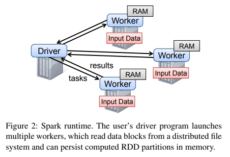
To use Spark, developers write a driver program that connects to a cluster of workers, as shown in Figure 2. The driver defines one or more RDDs and invokes actions on them. Spark code on the driver also tracks the RDDs’ lineage. The workers are long-lived processes that can store RDD partitions in RAM across operations.
Spark를 사용하려면 개발자는 그림 2와 같이 워커 클러스터에 연결하는 드라이버 프로그램을 작성해야 한다. 드라이버는 하나 이상의 RDD를 정의하고, 그에 대한 액션을 호출한다. 또한, 드라이버에서 실행되는 Spark 코드는 RDD의 계보를 추적한다. 워커는 장기간 실행되는 프로세스로, 여러 연산에 걸쳐 RDD 파티션을 RAM에 저장할 수 있다.
As we showed in the log mining example in Section 2.2.1, users provide arguments to RDD operations like map by passing closures (function literals). Scala represents each closure as a Java object, and these objects can be serialized and loaded on another node to pass the closure across the network. Scala also saves any variables bound in the closure as fields in the Java object. For example, one can write code like var x = 5; rdd.map(_ + x) to add 5 to each element of an RDD.5
섹션 2.2.1의 로그 마이닝 예제에서 보여준 것처럼, 사용자는 map과 같은 RDD 연산에 클로저(함수 리터럴)를 전달하여 인수를 제공한다. Scala는 각 클로저를 Java 객체로 표현하며, 이러한 객체들은 직렬화되어 네트워크를 통해 다른 노드로 전송될 수 있다. 또한, Scala는 클로저 내에서 바인딩된 변수를 Java 객체의 필드로 저장한다. 예를 들어, var x = 5; rdd.map(_ + x)와 같은 코드를 작성하면, RDD의 각 요소에 5를 더할 수 있다.
RDDs themselves are statically typed objects parametrized by an element type. For example, RDD[Int] is an RDD of integers. However, most of our examples omit types since Scala supports type inference.
RDD 자체는 요소 타입을 매개변수로 하는 정적 타입 객체이다. 예를 들어, RDD[Int]는 정수형 요소를 가지는 RDD이다. 그러나 Scala는 타입 추론을 지원하므로, 대부분의 예제에서는 타입을 생략하고 있다.
Although our method of exposing RDDs in Scala is conceptually simple, we had to work around issues with Scala’s closure objects using reflection [33]. We also needed more work to make Spark usable from the Scala interpreter, as we shall discuss in Section 5.2. Nonetheless, we did not have to modify the Scala compiler.
비록 Scala에서 RDD를 노출하는 방식은 개념적으로 단순하지만, 우리는 Scala의 클로저 객체와 관련된 문제를 반사(reflection) [33]를 사용하여 해결해야 했다. 또한, Spark를 Scala 인터프리터에서 사용 가능하게 만들기 위해 추가적인 작업이 필요했으며, 이에 대해서는 섹션 5.2에서 논의할 것이다. 그럼에도 불구하고, 우리는 Scala 컴파일러를 수정할 필요는 없었다.
3.1 RDD Operations in Spark
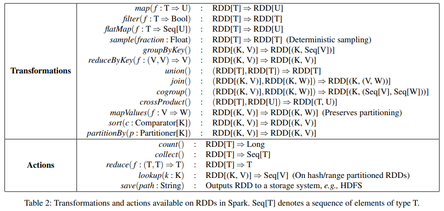
Table 2 lists the main RDD transformations and actions available in Spark. We give the signature of each operation, showing type parameters in square brackets. Recall that transformations are lazy operations that define a new RDD, while actions launch a computation to return a value to the program or write data to external storage.
표 2는 Spark에서 사용할 수 있는 주요 RDD 변환(transformations)과 액션(actions)을 나열한다. 각 연산의 시그니처를 제시하며, 타입 매개변수는 대괄호로 표시하였다. 변환은 새로운 RDD를 정의하는 지연 연산(lazy operations)인 반면, 액션은 값을 프로그램에 반환하거나 데이터를 외부 저장소에 기록하기 위해 연산을 실행한다는 점을 기억해야 한다.
Note that some operations, such as join, are only available on RDDs of key-value pairs. Also, our function names are chosen to match other APIs in Scala and other functional languages; for example, map is a one-to-one mapping, while flatMap maps each input value to one or more outputs (similar to the map in MapReduce).
일부 연산(join 등)은 키-값 쌍을 가진 RDD에서만 사용할 수 있다는 점에 유의해야 한다. 또한, 함수 이름은 Scala 및 기타 함수형 언어의 API와 일치하도록 선택되었다. 예를 들어, map은 1:1 매핑을 수행하는 반면, flatMap은 각 입력 값을 하나 이상의 출력으로 매핑하며, 이는 MapReduce의 map 연산과 유사하다.
In addition to these operators, users can ask for an RDD to persist. Furthermore, users can get an RDD’s partition order, which is represented by a Partitioner class, and partition another dataset according to it. Operations such as groupByKey, reduceByKey and sort automatically result in a hash or range partitioned RDD.
이러한 연산자 외에도, 사용자는 RDD의 지속성을 요청할 수 있다. 또한, RDD의 파티션 순서를 Partitioner 클래스를 통해 확인하고, 이를 기반으로 다른 데이터셋을 파티셔닝할 수도 있다. groupByKey, reduceByKey, sort와 같은 연산은 자동으로 해시 파티셔닝 또는 범위 파티셔닝된 RDD를 생성한다.
3.2 Example Applications
We complement the data mining example in Section 2.2.1 with two iterative applications: logistic regression and PageRank. The latter also showcases how control of RDDs’ partitioning can improve performance.
우리는 섹션 2.2.1의 데이터 마이닝 예제를 보완하기 위해 두 가지 반복적(iterative) 애플리케이션인 로지스틱 회귀(logistic regression)와 PageRank를 추가한다. 후자는 RDD의 파티셔닝을 제어함으로써 성능을 향상시킬 수 있는 방법을 보여준다.
3.2.1 Logistic Regression
Many machine learning algorithms are iterative in nature because they run iterative optimization procedures, such as gradient descent, to maximize a function. They can thus run much faster by keeping their data in memory.
많은 머신러닝 알고리즘은 반복적인 최적화 절차(예: 경사 하강법)를 실행하여 함수를 최적화하기 때문에 본질적으로 반복적인 특성을 가진다. 따라서, 이러한 알고리즘은 데이터를 메모리에 유지함으로써 훨씬 빠르게 실행될 수 있다.
As an example, the following program implements logistic regression [14], a common classification algorithm that searches for a hyperplane w that best separates two sets of points (e.g., spam and non-spam emails). The algorithm uses gradient descent: it starts w at a random value, and on each iteration, it sums a function of w over the data to move w in a direction that improves it.
예를 들어, 다음 프로그램은 로지스틱 회귀(logistic regression) [14]를 구현하며, 이는 두 개의 점 집합(예: 스팸 이메일과 비스팸 이메일)을 가장 잘 분리하는 초평면 w를 찾는 일반적인 분류 알고리즘이다. 이 알고리즘은 경사 하강법(gradient descent)을 사용하며, w를 임의의 값에서 시작한 후 각 반복(iteration)마다 데이터 전체에 걸쳐 w의 함수를 합산하여 w를 더 나은 방향으로 이동시킨다.
val points = spark.textFile(...)
.map(parsePoint)
.persist()
var w = // 랜덤 초기 벡터
for (i <- 1 to ITERATIONS) {
val gradient = points.map { p =>
p.x * (1 / (1 + exp(-p.y * (w dot p.x))) - 1) * p.y
}.reduce((a, b) => a + b)
w -= gradient
}
We start by defining a persistent RDD called points as the result of a map transformation on a text file that parses each line of text into a Point object. We then repeatedly run map and reduce on points to compute the gradient at each step by summing a function of the current w. Keeping points in memory across iterations can yield a 20× speedup, as we show in Section 6.1.
우리는 먼저 points라는 지속적인 RDD를 정의하는데, 이는 텍스트 파일에 map 변환을 적용하여 각 텍스트 라인을 Point 객체로 변환한 결과이다. 그런 다음, 각 단계에서 현재 w의 함수를 합산하여 그래디언트를 계산하기 위해 points에 대해 map과 reduce를 반복적으로 실행한다. 반복 과정에서 points를 메모리에 유지하면 최대 20배의 속도 향상을 얻을 수 있으며, 이에 대한 자세한 내용은 섹션 6.1에서 설명한다.
3.2.2 PageRank
A more complex pattern of data sharing occurs in PageRank [6]. The algorithm iteratively updates a rank for each document by adding up contributions from documents that link to it. On each iteration, each document sends a contribution of r n to its neighbors, where r is its rank and n is its number of neighbors. It then updates its rank to α/N + (1 − α)∑ci , where the sum is over the contributions it received and N is the total number of documents. We can write PageRank in Spark as follows:
PageRank [6]에서는 더 복잡한 형태의 데이터 공유 패턴이 발생한다. 이 알고리즘은 반복적으로 각 문서의 랭크를 업데이트하며, 이는 해당 문서로 연결된 문서들의 기여도를 합산하는 방식으로 이루어진다. 각 반복에서, 각 문서는 자신의 랭크 r을 이웃 문서 개수 n으로 나눈 값을 이웃들에게 기여도로 전달한다. 그런 다음, 랭크는 α/N + (1 − α)∑ci로 업데이트되는데, 여기서 합(sum)은 해당 문서가 받은 기여도를 의미하며, N은 전체 문서의 개수이다. Spark에서 PageRank를 다음과 같이 구현할 수 있다.
// (URL, outlinks) 쌍의 RDD로 그래프 로드
val links = spark.textFile(...).map(...).persist()
var ranks = // (URL, rank) 쌍의 RDD
for (i <- 1 to ITERATIONS) {
// 각 페이지가 보낸 기여도로 이루어진 (targetURL, float) 쌍의 RDD 생성
val contribs = links.join(ranks).flatMap {
case (url, (links, rank)) =>
links.map(dest => (dest, rank / links.size))
}
// URL별로 기여도를 합산하여 새로운 랭크 계산
ranks = contribs.reduceByKey((x, y) => x + y)
.mapValues(sum => a / N + (1 - a) * sum)
}

This program leads to the RDD lineage graph in Figure 3. On each iteration, we create a new ranks dataset based on the contribs and ranks from the previous iteration and the static links dataset.6 One interesting feature of this graph is that it grows longer with the number of iterations. Thus, in a job with many iterations, it may be necessary to reliably replicate some of the versions of ranks to reduce fault recovery times [20]. The user can call persist with a RELIABLE flag to do this. However, note that the links dataset does not need to be replicated, because partitions of it can be rebuilt efficiently by rerunning a map on blocks of the input file. This dataset will typically be much larger than ranks, because each document has many links but only one number as its rank, so recovering it using lineage saves time over systems that checkpoint a program’s entire in-memory state.
이 프로그램은 그림 3의 RDD 계보(lineage) 그래프를 생성한다. 각 반복에서 이전 반복의 contribs와 ranks, 그리고 변하지 않는 links 데이터셋을 기반으로 새로운 ranks 데이터셋을 만든다.
이 그래프의 흥미로운 특징 중 하나는 반복 횟수가 증가할수록 계보 그래프가 길어진다는 점이다. 따라서 반복 횟수가 많은 작업에서는 장애 복구 시간을 줄이기 위해 ranks의 일부 버전을 신뢰성 있게 복제(replicate)하는 것이 필요할 수 있다 [20]. 이를 위해 사용자는 persist 메서드를 호출할 때 RELIABLE 플래그를 설정할 수 있다.
그러나 links 데이터셋은 복제할 필요가 없다. 그 이유는 입력 파일의 블록에 대해 map 연산을 다시 실행하는 방식으로 해당 파티션을 효율적으로 재구성할 수 있기 때문이다. 또한, links 데이터셋은 일반적으로 ranks보다 훨씬 크다. 각 문서는 여러 개의 링크를 포함할 수 있지만, ranks는 각 문서에 대해 단 하나의 숫자만 저장하기 때문이다. 따라서, 계보(lineage)를 활용한 복구 방식은 프로그램의 전체 메모리 상태를 체크포인트(checkpoint)하는 기존 시스템보다 복구 시간을 절약할 수 있다.
Finally, we can optimize communication in PageRank by controlling the partitioning of the RDDs. If we specify a partitioning for links (e.g., hash-partition the link lists by URL across nodes), we can partition ranks in the same way and ensure that the join operation between links and ranks requires no communication (as each URL’s rank will be on the same machine as its link list). We can also write a custom Partitioner class to group pages that link to each other together (e.g., partition the URLs by domain name). Both optimizations can be expressed by calling partitionBy when we define links:
마지막으로, RDD의 파티셔닝을 제어함으로써 PageRank에서의 통신을 최적화할 수 있다. 예를 들어, links에 대해 특정한 파티셔닝을 지정하면(예: URL을 기준으로 링크 목록을 해시 파티셔닝하여 여러 노드에 분배), ranks를 동일한 방식으로 파티셔닝할 수 있다. 이렇게 하면 links와 ranks 간의 join 연산에서 통신이 필요하지 않게 되며, 각 URL의 랭크가 해당 링크 목록과 동일한 머신에 위치하게 된다.
또한, 맞춤형 Partitioner 클래스를 작성하여 서로 연결된 페이지들을 같은 그룹으로 묶을 수도 있다(예: 도메인 이름을 기준으로 URL을 파티셔닝). 이러한 최적화 기법들은 links를 정의할 때 partitionBy 메서드를 호출하여 적용할 수 있다.
links = spark.textFile(...).map(...).partitionBy(myPartFunc).persist()
After this initial call, the join operation between links and ranks will automatically aggregate the contributions for each URL to the machine that its link lists is on, calculate its new rank there, and join it with its links. This type of consistent partitioning across iterations is one of the main optimizations in specialized frameworks like Pregel. RDDs let the user express this goal directly.
이 초기 호출 이후, links와 ranks 간의 join 연산은 각 URL의 링크 목록이 위치한 머신으로 자동으로 기여도를 집계하고, 해당 머신에서 새로운 랭크를 계산한 후 이를 링크와 결합하게 된다.
이러한 일관된 파티셔닝 방식은 Pregel과 같은 특화된 프레임워크에서 사용되는 주요 최적화 기법 중 하나이다. RDD를 사용하면 사용자가 이러한 목표를 직접 표현할 수 있다.
4 Representing RDDs
One of the challenges in providing RDDs as an abstraction is choosing a representation for them that can track lineage across a wide range of transformations. Ideally, a system implementing RDDs should provide as rich a set of transformation operators as possible (e.g., the ones in Table 2), and let users compose them in arbitrary ways. We propose a simple graph-based representation for RDDs that facilitates these goals. We have used this representation in Spark to support a wide range of transformations without adding special logic to the scheduler for each one, which greatly simplified the system design.
RDD를 추상화로 제공하는 데 있어서의 도전 과제 중 하나는 다양한 변환(transformations)에 걸쳐 lineage(계보)를 추적할 수 있는 표현 방식을 선택하는 것이다. 이상적으로, RDD를 구현하는 시스템은 가능한 한 풍부한 변환 연산자 집합(예: 표 2에 나열된 것들)을 제공하고, 사용자가 이를 임의의 방식으로 조합할 수 있도록 해야 한다. 우리는 이러한 목표를 용이하게 하는 간단한 그래프 기반 표현 방식을 RDD에 대해 제안한다. 우리는 이 표현 방식을 Spark에서 사용하여 스케줄러에 각 변환을 위한 특별한 로직을 추가하지 않고도 다양한 변환을 지원할 수 있었으며, 이는 시스템 설계를 크게 단순화했다.

In a nutshell, we propose representing each RDD through a common interface that exposes five pieces of information: a set of partitions, which are atomic pieces of the dataset; a set of dependencies on parent RDDs; a function for computing the dataset based on its parents; and metadata about its partitioning scheme and data placement. For example, an RDD representing an HDFS file has a partition for each block of the file and knows which machines each block is on. Meanwhile, the result of a map on this RDD has the same partitions, but applies the map function to the parent’s data when computing its elements. We summarize this interface in Table 3.
간단히 말해, 우리는 각 RDD를 다섯 가지 정보를 노출하는 공통 인터페이스를 통해 표현하는 것을 제안한다: 데이터셋의 원자적 조각인 파티션(partitions) 집합, 부모 RDD에 대한 의존성(dependencies) 집합, 부모를 기반으로 데이터셋을 계산하기 위한 함수(function), 그리고 파티셔닝 방식(partitioning scheme)과 데이터 배치(data placement)에 대한 메타데이터(metadata). 예를 들어, HDFS 파일을 나타내는 RDD는 파일의 각 블록에 대해 하나의 파티션을 가지며, 각 블록이 어떤 머신에 위치하는지 알고 있다. 한편, 이 RDD에 대한 map 연산의 결과는 동일한 파티션을 가지지만, 요소를 계산할 때 부모의 데이터에 map 함수를 적용한다. 우리는 이 인터페이스를 표 3에 요약하였다.
The most interesting question in designing this interface is how to represent dependencies between RDDs. We found it both sufficient and useful to classify dependencies into two types: narrow dependencies, where each partition of the parent RDD is used by at most one partition of the child RDD, wide dependencies, where multiple child partitions may depend on it. For example, map leads to a narrow dependency, while join leads to to wide dependencies (unless the parents are hash-partitioned). Figure 4 shows other examples.
이 인터페이스를 설계하는 데 있어 가장 흥미로운 질문은 RDD 간의 의존성을 어떻게 표현할 것인가이다.
우리는 의존성을 두 가지 유형으로 분류하는 것이 충분하며 유용하다는 사실을 발견했다: 첫째, 좁은 의존성(narrow dependencies)으로, 부모 RDD의 각 파티션이 자식 RDD의 최대 한 개 파티션에서 사용되는 경우이며, 둘째, 넓은 의존성(wide dependencies)으로, 여러 자식 파티션이 하나의 부모 파티션에 의존할 수 있는 경우이다. 예를 들어, map 연산은 좁은 의존성을 초래하는 반면, join 연산은 넓은 의존성을 초래한다(부모 RDD가 해시 파티셔닝된 경우가 아니라면). 그림 4는 다른 예시를 보여준다.

This distinction is useful for two reasons. First, narrow dependencies allow for pipelined execution on one cluster node, which can compute all the parent partitions. For example, one can apply a map followed by a filter on an element-by-element basis. In contrast, wide dependencies require data from all parent partitions to be available and to be shuffled across the nodes using a MapReducelike operation. Second, recovery after a node failure is more efficient with a narrow dependency, as only the lost parent partitions need to be recomputed, and they can be recomputed in parallel on different nodes. In contrast, in a lineage graph with wide dependencies, a single failed node might cause the loss of some partition from all the ancestors of an RDD, requiring a complete re-execution.
이 구분은 두 가지 이유로 유용하다. 첫째, 좁은 의존성(narrow dependencies)은 하나의 클러스터 노드에서 파이프라인 실행을 가능하게 하며, 이는 모든 부모 파티션을 계산할 수 있다. 예를 들어, 요소별로 map 연산을 적용한 후 filter 연산을 적용할 수 있다. 반면, 넓은 의존성(wide dependencies)은 모든 부모 파티션의 데이터가 필요하며, MapReduce와 유사한 연산을 통해 노드 간에 데이터를 셔플(shuffle)해야 한다. 둘째, 좁은 의존성은 노드 장애 후 복구가 더 효율적이다. 손실된 부모 파티션만 재계산하면 되며, 서로 다른 노드에서 병렬로 재계산할 수 있다. 반면, 넓은 의존성이 있는 lineage 그래프에서는 단일 노드의 장애로 인해 RDD의 모든 조상(ancestors)으로부터 일부 파티션이 손실될 수 있으며, 이는 완전한 재실행을 필요로 할 수 있다.
This common interface for RDDs made it possible to implement most transformations in Spark in less than 20 lines of code. Indeed, even new Spark users have implemented new transformations (e.g., sampling and various types of joins) without knowing the details of the scheduler. We sketch some RDD implementations below.
RDD에 대한 이 공통 인터페이스는 Spark에서 대부분의 변환(transformations)을 20줄 이하의 코드로 구현할 수 있게 했다. 실제로, 새로운 Spark 사용자들도 스케줄러의 세부 사항을 알지 못한 상태에서 새로운 변환(예: 샘플링 및 다양한 유형의 조인)을 구현했다. 아래에서 몇 가지 RDD 구현을 간략히 설명한다.
HDFS files: The input RDDs in our samples have been files in HDFS. For these RDDs, partitions returns one partition for each block of the file (with the block’s offset stored in each Partition object), preferredLocations gives the nodes the block is on, and iterator reads the block.
HDFS 파일: 우리의 샘플에서 입력 RDD는 HDFS 파일이었다. 이러한 RDD의 경우, partitions는 파일의 각 블록에 대해 하나의 파티션을 반환하며(각 Partition 객체에 블록의 오프셋이 저장됨), preferredLocations는 블록이 위치한 노드를 제공하고, iterator는 블록을 읽는다.
map: Calling map on any RDD returns a MappedRDD object. This object has the same partitions and preferred locations as its parent, but applies the function passed to map to the parent’s records in its iterator method.
map: 어떤 RDD에 대해 map을 호출하면 MappedRDD 객체가 반환된다. 이 객체는 부모와 동일한 파티션과 preferredLocations를 가지지만, iterator 메서드에서 부모의 레코드에 map에 전달된 함수를 적용한다.
union: Calling union on two RDDs returns an RDD whose partitions are the union of those of the parents. Each child partition is computed through a narrow dependency on the corresponding parent.
* Note that our union operation does not drop duplicate values.
* 참고로, 우리의 union 연산은 중복 값을 제거하지 않는다.
union: 두 RDD에 대해 union을 호출하면 부모 RDD의 파티션들을 합친 RDD가 반환된다. 각 자식 파티션은 해당 부모에 대한 좁은 의존성(narrow dependency)을 통해 계산된다.
sample: Sampling is similar to mapping, except that the RDD stores a random number generator seed for each partition to deterministically sample parent records.
sample: 샘플링은 매핑과 유사하지만, RDD는 각 파티션에 대해 난수 생성기 시드를 저장하여 부모 레코드를 결정적으로(deterministically) 샘플링한다.
join: Joining two RDDs may lead to either two narrow dependencies (if they are both hash/range partitioned with the same partitioner), two wide dependencies, or a mix (if one parent has a partitioner and one does not). In either case, the output RDD has a partitioner (either one inherited from the parents or a default hash partitioner).
join: 두 RDD를 조인(join)하면 두 개의 좁은 의존성(둘 다 동일한 파티셔너로 해시/범위 파티셔닝된 경우), 두 개의 넓은 의존성(wide dependencies), 또는 혼합(한 부모는 파티셔너가 있고 다른 한 부모는 없는 경우)이 발생할 수 있다. 어느 경우든, 출력 RDD는 파티셔너를 가진다(부모로부터 상속받은 파티셔너 또는 기본 해시 파티셔너).
5 Implementation
We have implemented Spark in about 14,000 lines of Scala. The system runs over the Mesos cluster manager [17], allowing it to share resources with Hadoop, MPI and other applications. Each Spark program runs as a separate Mesos application, with its own driver (master) and workers, and resource sharing between these applications is handled by Mesos.
우리는 Spark를 약 14,000줄의 Scala 코드로 구현했다. 이 시스템은 Mesos 클러스터 관리자 위에서 동작하며, 이를 통해 Hadoop, MPI 및 다른 애플리케이션과 자원을 공유할 수 있다. 각 Spark 프로그램은 별도의 Mesos 애플리케이션으로 실행되며, 자체적인 드라이버(마스터)와 작업자(workers)를 가지고 있다. 이러한 애플리케이션 간의 자원 공유는 Mesos가 처리한다.
Spark can read data from any Hadoop input source (e.g., HDFS or HBase) using Hadoop’s existing input plugin APIs, and runs on an unmodified version of Scala.
Spark는 Hadoop의 기존 입력 플러그인 API를 사용하여 모든 Hadoop 입력 소스(예: HDFS 또는 HBase)에서 데이터를 읽을 수 있으며, 수정되지 않은 Scala 버전에서 실행된다.
We now sketch several of the technically interesting parts of the system: our job scheduler (§5.1), our Spark interpreter allowing interactive use (§5.2), memory management (§5.3), and support for checkpointing (§5.4).
이제 시스템의 기술적으로 흥미로운 부분 중 몇 가지를 간략히 설명한다: 작업 스케줄러(§5.1), 대화형 사용을 가능하게 하는 Spark 인터프리터(§5.2), 메모리 관리(§5.3), 그리고 체크포인팅 지원(§5.4).
5.1 Job Scheduling
Spark’s scheduler uses our representation of RDDs, described in Section 4.
Spark의 스케줄러는 4절에서 설명한 RDD 표현 방식을 사용한다.

Overall, our scheduler is similar to Dryad’s [19], but it additionally takes into account which partitions of persistent RDDs are available in memory. Whenever a user runs an action (e.g., count or save) on an RDD, the scheduler examines that RDD’s lineage graph to build a DAG of stages to execute, as illustrated in Figure 5. Each stage contains as many pipelined transformations with narrow dependencies as possible. The boundaries of the stages are the shuffle operations required for wide dependencies, or any already computed partitions that can shortcircuit the computation of a parent RDD. The scheduler then launches tasks to compute missing partitions from each stage until it has computed the target RDD.
전체적으로, 우리의 스케줄러는 Dryad의 스케줄러와 유사하지만, 영구적인(persistent) RDD의 어떤 파티션이 메모리에 있는지도 추가적으로 고려한다. 사용자가 RDD에 대해 액션(예: count 또는 save)을 실행할 때마다, 스케줄러는 해당 RDD의 lineage 그래프를 검토하여 실행할 단계(stage)의 DAG(방향성 비순환 그래프)를 구축한다. 이는 그림 5에 설명되어 있다. 각 단계는 가능한 한 많은 좁은 의존성(narrow dependencies)을 가진 파이프라인 변환을 포함한다. 단계의 경계는 넓은 의존성(wide dependencies)을 위한 셔플(shuffle) 연산이거나, 부모 RDD의 계산을 단축할 수 있는 이미 계산된 파티션이다. 그런 다음 스케줄러는 각 단계에서 누락된 파티션을 계산하기 위해 작업(task)을 시작하고, 목표 RDD가 계산될 때까지 진행한다.
Our scheduler assigns tasks to machines based on data locality using delay scheduling [32]. If a task needs to process a partition that is available in memory on a node, we send it to that node. Otherwise, if a task processes a partition for which the containing RDD provides preferred locations (e.g., an HDFS file), we send it to those.
우리의 스케줄러는 지연 스케줄링(delay scheduling)을 사용하여 데이터 지역성(data locality)을 기반으로 작업(task)을 머신에 할당한다. 만약 작업이 특정 노드의 메모리에 있는 파티션을 처리해야 한다면, 해당 작업을 그 노드로 보낸다. 그렇지 않고, 작업이 특정 RDD의 파티션을 처리해야 하며 해당 RDD가 선호 위치(preferred locations)를 제공하는 경우(예: HDFS 파일), 작업을 그 위치로 보낸다.
For wide dependencies (i.e., shuffle dependencies), we currently materialize intermediate records on the nodes holding parent partitions to simplify fault recovery, much like MapReduce materializes map outputs.
넓은 의존성(wide dependencies), 즉 셔플 의존성(shuffle dependencies)의 경우, 현재 우리는 장애 복구를 단순화하기 위해 부모 파티션을 보유한 노드에서 중간 레코드를 구체화(materialize)한다. 이는 MapReduce가 맵 출력을 구체화하는 방식과 매우 유사하다.
If a task fails, we re-run it on another node as long as its stage’s parents are still available. If some stages have become unavailable (e.g., because an output from the “map side” of a shuffle was lost), we resubmit tasks to compute the missing partitions in parallel. We do not yet tolerate scheduler failures, though replicating the RDD lineage graph would be straightforward.
작업(task)이 실패하면, 해당 단계(stage)의 부모가 여전히 사용 가능한 한 다른 노드에서 작업을 다시 실행한다. 만약 일부 단계가 사용 불가능해진 경우(예: 셔플(shuffle)의 "맵 측면" 출력이 손실된 경우), 누락된 파티션을 계산하기 위해 작업을 다시 제출하고 병렬로 처리한다. 아직 스케줄러 장애를 허용하지는 않지만, RDD lineage 그래프를 복제하는 것은 간단할 것이다.
Finally, although all computations in Spark currently run in response to actions called in the driver program, we are also experimenting with letting tasks on the cluster (e.g., maps) call the lookup operation, which provides random access to elements of hash-partitioned RDDs by key. In this case, tasks would need to tell the scheduler to compute the required partition if it is missing.
마지막으로, 현재 Spark의 모든 계산은 드라이버 프로그램에서 호출된 액션에 응답하여 실행되지만, 클러스터의 작업(예: 맵)이 lookup 연산을 호출할 수 있도록 하는 실험도 진행 중이다. 이 연산은 키(key)를 통해 해시 파티셔닝된 RDD의 요소에 무작위 접근을 제공한다. 이 경우, 작업은 필요한 파티션이 누락된 경우 스케줄러에게 해당 파티션을 계산하도록 요청해야 한다.
5.2 Interpreter Integration
Scala includes an interactive shell similar to those of Ruby and Python. Given the low latencies attained with in-memory data, we wanted to let users run Spark interactively from the interpreter to query big datasets.
Scala는 Ruby와 Python의 인터랙티브 셸과 유사한 인터랙티브 셸을 포함한다. 메모리 내 데이터로 달성된 낮은 지연 시간을 고려하여, 우리는 사용자가 인터프리터를 통해 Spark를 대화형으로 실행하여 대규모 데이터셋을 쿼리할 수 있도록 하고 싶었다.
The Scala interpreter normally operates by compiling a class for each line typed by the user, loading it into the JVM, and invoking a function on it. This class includes a singleton object that contains the variables or functions on that line and runs the line’s code in an initialize method. For example, if the user types var x = 5 followed by println(x), the interpreter defines a class called Line1 containing x and causes the second line to compile to println(Line1.getInstance().x).
Scala 인터프리터는 일반적으로 사용자가 입력한 각 줄에 대해 클래스를 컴파일한 후 이를 JVM에 로드하고, 해당 클래스에서 함수를 호출하는 방식으로 동작한다. 이 클래스는 단일 객체(singleton object)를 포함하며, 해당 줄의 변수를 저장하거나 함수를 정의한 후, initialize 메서드에서 해당 줄의 코드를 실행한다. 예를 들어, 사용자가 var x = 5를 입력한 후 println(x)를 입력하면, 인터프리터는 x를 포함하는 Line1이라는 클래스를 정의하고, 두 번째 줄을 println(Line1.getInstance().x)로 컴파일한다.
We made two changes to the interpreter in Spark:
Spark에서는 인터프리터에 두 가지 변경을 적용했다.
1. Class shipping: To let the worker nodes fetch the bytecode for the classes created on each line, we made the interpreter serve these classes over HTTP.
1. 클래스 전송(Class shipping): 각 줄에서 생성된 클래스의 바이트코드를 워커 노드에서 가져올 수 있도록, 인터프리터가 HTTP를 통해 해당 클래스를 제공하도록 만들었다.
2. Modified code generation: Normally, the singleton object created for each line of code is accessed through a static method on its corresponding class. This means that when we serialize a closure referencing a variable defined on a previous line, such as Line1.x in the example above, Java will not trace through the object graph to ship the Line1 instance wrapping around x. Therefore, the worker nodes will not receive x. We modified the code generation logic to reference the instance of each line object directly.
수정된 코드 생성(Modified code generation): 일반적으로 각 코드 줄에서 생성된 단일 객체(singleton object)는 해당 클래스의 정적(static) 메서드를 통해 접근된다. 따라서, 만약 클로저가 이전 줄에서 정의된 변수(예: Line1.x)를 참조할 경우, Java는 객체 그래프를 따라가면서 Line1 인스턴스를 추적하지 않으므로, 워커 노드가 x 값을 받을 수 없다. 이를 해결하기 위해 코드 생성 로직을 수정하여, 각 줄에서 생성된 객체의 인스턴스를 직접 참조하도록 변경했다.

Figure 6 shows how the interpreter translates a set of lines typed by the user to Java objects after our changes.
그림 6은 인터프리터가 사용자가 입력한 여러 줄의 코드를 우리의 변경 사항을 적용한 후 Java 객체로 변환하는 과정을 보여준다.
We found the Spark interpreter to be useful in processing large traces obtained as part of our research and exploring datasets stored in HDFS. We also plan to use to run higher-level query languages interactively, e.g., SQL.
우리는 Spark 인터프리터가 연구 과정에서 얻은 대규모 트레이스를 처리하고, HDFS에 저장된 데이터셋을 탐색하는 데 유용하다는 것을 확인했다. 또한, SQL과 같은 고수준의 질의 언어를 대화형으로 실행하는 데에도 활용할 계획이다.
5.3 Memory Management
Spark provides three options for storage of persistent RDDs: in-memory storage as deserialized Java objects, in-memory storage as serialized data, and on-disk storage. The first option provides the fastest performance, because the Java VM can access each RDD element natively. The second option lets users choose a more memory-efficient representation than Java object graphs when space is limited, at the cost of lower performance.* The third option is useful for RDDs that are too large to keep in RAM but costly to recompute on each use.
Spark는 지속적인 RDD를 저장하는 세 가지 옵션을 제공한다. 첫 번째 옵션은 역직렬화된(deserialized) Java 객체로 메모리에 저장하는 방식으로, Java VM이 각 RDD 요소에 직접 접근할 수 있어 가장 빠른 성능을 제공한다.
두 번째 옵션은 직렬화된(serialized) 데이터로 메모리에 저장하는 방식으로, 메모리 공간이 제한적일 때 Java 객체 그래프보다 더 효율적인 표현을 사용할 수 있지만, 성능은 낮아진다.
세 번째 옵션은 RDD를 디스크에 저장하는 방식으로, RAM에 유지하기에는 너무 크지만, 사용할 때마다 다시 계산하는 것이 비용이 많이 드는 RDD에 유용하다.
* The cost depends on how much computation the application does per byte of data, but can be up to 2× for lightweight processing.
비용은 애플리케이션이 데이터의 바이트당 수행하는 연산량에 따라 달라지지만, 연산이 가벼운 경우 최대 2배까지 증가할 수 있다.
To manage the limited memory available, we use an LRU eviction policy at the level of RDDs. When a new RDD partition is computed but there is not enough space to store it, we evict a partition from the least recently accessed RDD, unless this is the same RDD as the one with the new partition. In that case, we keep the old partition in memory to prevent cycling partitions from the same RDD in and out. This is important because most operations will run tasks over an entire RDD, so it is quite likely that the partition already in memory will be needed in the future. We found this default policy to work well in all our applications so far, but we also give users further control via a “persistence priority” for each RDD.
한정된 메모리를 효과적으로 관리하기 위해, 우리는 RDD 단위에서 LRU(Least Recently Used) 제거 정책을 사용한다. 새로운 RDD 파티션을 계산할 때 저장할 공간이 부족하면, 가장 오랫동안 접근되지 않은 RDD에서 파티션을 제거한다. 단, 새로운 파티션이 생성된 RDD와 같은 RDD에서 제거할 경우에는 기존 파티션을 메모리에 유지한다.
이러한 방식은 동일한 RDD의 파티션이 메모리에서 반복적으로 제거되고 다시 로드되는 사이클링 문제를 방지하는 데 중요하다. 대부분의 연산은 전체 RDD에 대해 실행되므로, 메모리에 이미 있는 파티션이 이후에도 필요할 가능성이 높기 때문이다.
우리는 이 기본 정책이 지금까지 모든 애플리케이션에서 효과적으로 작동함을 확인했으며, 추가적으로 사용자가 각 RDD에 대해 "지속성 우선순위(persistence priority)"를 설정하여 보다 세밀하게 제어할 수 있도록 지원한다.
Finally, each instance of Spark on a cluster currently has its own separate memory space. In future work, we plan to investigate sharing RDDs across instances of Spark through a unified memory manager.
현재 클러스터에서 실행되는 각 Spark 인스턴스는 개별적인 메모리 공간을 사용한다. 향후 연구에서는 통합 메모리 관리 시스템을 통해 여러 Spark 인스턴스 간에 RDD를 공유하는 방안을 연구할 계획이다.
5.4 Support for Checkpointing
Although lineage can always be used to recover RDDs after a failure, such recovery may be time-consuming for RDDs with long lineage chains. Thus, it can be helpful to checkpoint some RDDs to stable storage.
계보(lineage)를 사용하면 항상 장애 이후 RDD를 복구할 수 있지만, 계보 체인이 길어진 RDD의 경우 이러한 복구 과정이 시간이 많이 소요될 수 있다. 따라서 일부 RDD를 안정적인 저장소에 체크포인트하는 것이 도움이 될 수 있다.
In general, checkpointing is useful for RDDs with long lineage graphs containing wide dependencies, such as the rank datasets in our PageRank example (§3.2.2). In these cases, a node failure in the cluster may result in the loss of some slice of data from each parent RDD, requiring a full recomputation [20]. In contrast, for RDDs with narrow dependencies on data in stable storage, such as the points in our logistic regression example (§3.2.1) and the link lists in PageRank, checkpointing may never be worthwhile. If a node fails, lost partitions from these RDDs can be recomputed in parallel on other nodes, at a fraction of the cost of replicating the whole RDD.
일반적으로, 체크포인트는 계보 그래프가 길고 광범위한 종속성을 가진 RDD에 유용하다. 예를 들어, PageRank 예제(§3.2.2)의 ranks 데이터셋이 이에 해당한다. 이러한 경우, 클러스터에서 노드 장애가 발생하면 각 부모 RDD의 일부 데이터가 손실될 수 있으며, 이로 인해 전체 RDD를 다시 계산해야 할 수도 있다.
반면, 안정적인 저장소에 있는 데이터에 대해 좁은 종속성을 가지는 RDD의 경우, 체크포인트가 거의 필요하지 않을 수 있다. 예를 들어, 로지스틱 회귀 예제(§3.2.1)의 points 데이터셋이나 PageRank의 links 리스트가 이에 해당한다. 이러한 RDD의 손실된 파티션은 다른 노드에서 병렬로 다시 계산할 수 있으며, 전체 RDD를 복제하는 것보다 훨씬 적은 비용이 든다.
Spark currently provides an API for checkpointing (a REPLICATE flag to persist), but leaves the decision of which data to checkpoint to the user. However, we are also investigating how to perform automatic checkpointing. Because our scheduler knows the size of each dataset as well as the time it took to first compute it, it should be able to select an optimal set of RDDs to checkpoint to minimize system recovery time [30].
Spark는 현재 체크포인트를 위한 API를 제공하며, 이를 위해 persist 메서드에서 REPLICATE 플래그를 사용할 수 있다. 그러나 어떤 데이터를 체크포인트할지는 사용자에게 맡긴다.
하지만 우리는 자동 체크포인트를 수행하는 방법도 연구하고 있다. 스케줄러는 각 데이터셋의 크기와 최초 계산에 소요된 시간을 알고 있으므로, 시스템 복구 시간을 최소화할 수 있도록 최적의 RDD 집합을 선택하여 체크포인트할 수 있을 것이다.
Finally, note that the read-only nature of RDDs makes them simpler to checkpoint than general shared memory. Because consistency is not a concern, RDDs can be written out in the background without requiring program pauses or distributed snapshot schemes.
마지막으로, RDD는 읽기 전용이므로 일반적인 공유 메모리보다 체크포인트가 더 간단하다. 일관성을 유지할 필요가 없기 때문에, 프로그램을 일시 중지하거나 분산 스냅샷 기법을 사용할 필요 없이 백그라운드에서 데이터를 기록할 수 있다.
6 Evaluation
We evaluated Spark and RDDs through a series of experiments on Amazon EC2, as well as benchmarks of user applications. Overall, our results show the following:
우리는 Amazon EC2에서 일련의 실험과 사용자 애플리케이션 벤치마크를 통해 Spark와 RDD를 평가했다. 전체적으로, 우리의 결과는 다음을 보여준다.
- Spark outperforms Hadoop by up to 20× in iterative machine learning and graph applications. The speedup comes from avoiding I/O and deserialization costs by storing data in memory as Java objects.
- Applications written by our users perform and scale well. In particular, we used Spark to speed up an analytics report that was running on Hadoop by 40×.
- When nodes fail, Spark can recover quickly by rebuilding only the lost RDD partitions.
- Spark can be used to query a 1 TB dataset interactively with latencies of 5–7 seconds.
- Spark는 반복적인 머신러닝 및 그래프 애플리케이션에서 Hadoop보다 최대 20배 빠른 성능을 보인다. 이러한 속도 향상은 데이터를 메모리에 Java 객체로 저장하여 I/O 및 역직렬화 비용을 피할 수 있기 때문이다.
- 사용자들이 작성한 애플리케이션도 높은 성능과 확장성을 보인다. 특히, Spark를 사용하여 Hadoop에서 실행되던 분석 보고서를 40배 빠르게 처리할 수 있었다.
- 노드 장애 발생 시, Spark는 손실된 RDD 파티션만 재구성하여 빠르게 복구할 수 있다.
- Spark는 1TB 규모의 데이터셋을 대화형으로 질의할 수 있으며, 지연 시간은 5~7초 정도이다.
We start by presenting benchmarks for iterative machine learning applications (§6.1) and PageRank (§6.2) against Hadoop. We then evaluate fault recovery in Spark (§6.3) and behavior when a dataset does not fit in memory (§6.4). Finally, we discuss results for user applications (§6.5) and interactive data mining (§6.6).
우리는 먼저 반복적인 머신러닝 애플리케이션(§6.1)과 PageRank(§6.2)에 대한 벤치마크를 수행하여 Hadoop과 비교한다. 이후, Spark의 장애 복구 성능(§6.3)과 데이터셋이 메모리에 맞지 않을 때의 동작 방식(§6.4)을 평가한다. 마지막으로, 사용자 애플리케이션(§6.5) 및 대화형 데이터 마이닝(§6.6)에 대한 결과를 논의한다.
Unless otherwise noted, our tests used m1.xlarge EC2 nodes with 4 cores and 15 GB of RAM. We used HDFS for storage, with 256 MB blocks. Before each test, we cleared OS buffer caches to measure IO costs accurately.
별도의 언급이 없는 한, 우리의 테스트는 4코어와 15GB RAM을 가진 m1.xlarge EC2 노드를 사용했으며, 저장소로는 HDFS(256MB 블록 크기)를 활용했다. 또한, I/O 비용을 정확하게 측정하기 위해 각 테스트 전에 OS 버퍼 캐시를 초기화했다.
6.1 Iterative Machine Learning Applications
We implemented two iterative machine learning applications, logistic regression and k-means, to compare the performance of the following systems:
우리는 로지스틱 회귀(logistic regression)와 K-means라는 두 개의 반복적인 머신러닝 애플리케이션을 구현하여 다음 시스템들의 성능을 비교했다.
- Hadoop: The Hadoop 0.20.2 stable release.
- HadoopBinMem: A Hadoop deployment that converts the input data into a low-overhead binary format in the first iteration to eliminate text parsing in later ones, and stores it in an in-memory HDFS instance.
- Spark: Our implementation of RDDs.
- Hadoop: Hadoop 0.20.2 안정 버전
- HadoopBinMem: 첫 번째 반복에서 입력 데이터를 오버헤드가 낮은 이진 형식(binary format)으로 변환하여 이후 반복에서 텍스트 파싱을 제거하고, 이를 인메모리 HDFS에 저장하는 Hadoop 배포 방식
- Spark: RDD를 활용한 우리의 구현
We ran both algorithms for 10 iterations on 100 GB datasets using 25–100 machines. The key difference between the two applications is the amount of computation they perform per byte of data. The iteration time of kmeans is dominated by computation, while logistic regression is less compute-intensive and thus more sensitive to time spent in deserialization and I/O.
우리는 두 알고리즘을 100GB 데이터셋을 사용하여 25–100대의 머신에서 10번의 반복을 실행했다. 두 애플리케이션의 주요 차이점은 데이터 바이트당 수행하는 연산량이다. K-means의 반복 시간은 주로 연산에 의해 결정되며, 반면 로지스틱 회귀는 연산 집약성이 낮아 역직렬화 및 I/O에 소요되는 시간에 더 민감하다.
Since typical learning algorithms need tens of iterations to converge, we report times for the first iteration and subsequent iterations separately. We find that sharing data via RDDs greatly speeds up future iterations.
일반적인 학습 알고리즘은 수십 번의 반복을 거쳐 수렴하기 때문에, 우리는 첫 번째 반복과 이후 반복의 시간을 별도로 보고한다. 우리는 RDD를 통해 데이터를 공유하면 이후 반복이 크게 가속화됨을 확인했다.
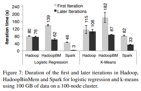
First Iterations: All three systems read text input from HDFS in their first iterations. As shown in the light bars in Figure 7, Spark was moderately faster than Hadoop across experiments. This difference was due to signaling overheads in Hadoop’s heartbeat protocol between its master and workers. HadoopBinMem was the slowest because it ran an extra MapReduce job to convert the data to binary, it and had to write this data across the network to a replicated in-memory HDFS instance.
첫 번째 반복에서 세 시스템 모두 HDFS에서 텍스트 입력을 읽는다. 그림 7의 밝은 색 막대에서 볼 수 있듯이, Spark는 모든 실험에서 Hadoop보다 다소 빠른 성능을 보였다. 이러한 차이는 Hadoop의 마스터와 워커 간 하트비트(heartbeat) 프로토콜에서 발생하는 신호 전달 오버헤드 때문이었다. HadoopBinMem은 데이터를 바이너리 형식으로 변환하는 추가적인 MapReduce 작업을 실행해야 했으며, 이 데이터를 네트워크를 통해 복제된 인메모리 HDFS 인스턴스로 저장해야 했기 때문에 가장 느렸다.

Subsequent Iterations: Figure 7 also shows the average running times for subsequent iterations, while Figure 8 shows how these scaled with cluster size. For logistic regression, Spark 25.3× and 20.7× faster than Hadoop and HadoopBinMem respectively on 100 machines. For the more compute-intensive k-means application, Spark still achieved speedup of 1.9× to 3.2×.
이후 반복에 대한 실행 시간 평균은 그림 7에, 클러스터 크기에 따른 확장성은 그림 8에 나타나 있다. 로지스틱 회귀의 경우, Spark는 100대의 머신에서 Hadoop보다 25.3배, HadoopBinMem보다 20.7배 빠른 성능을 보였다. 연산 집약적인 K-means 애플리케이션에서도 Spark는 1.9배에서 3.2배의 속도 향상을 달성했다.
Understanding the Speedup: We were surprised to find that Spark outperformed even Hadoop with inmemory storage of binary data (HadoopBinMem) by a 20× margin. In HadoopBinMem, we had used Hadoop’s standard binary format (SequenceFile) and a large block size of 256 MB, and we had forced HDFS’s data directory to be on an in-memory file system. However, Hadoop still ran slower due to several factors:
속도 향상의 원인 분석에서, 우리는 Spark가 인메모리 바이너리 데이터를 사용하는 HadoopBinMem보다도 20배 빠른 성능을 보였다는 점에 놀랐다. HadoopBinMem에서는 Hadoop의 표준 바이너리 포맷(SequenceFile)을 사용했으며, 256MB의 큰 블록 크기를 설정하고, HDFS의 데이터 디렉토리를 인메모리 파일 시스템에서 강제로 실행했다. 그러나 Hadoop은 여전히 여러 가지 요인으로 인해 더 느리게 실행되었다.
- Minimum overhead of the Hadoop software stack,
- Overhead of HDFS while serving data, and
- Deserialization cost to convert binary records to usable in-memory Java objects.
- Hadoop 소프트웨어 스택의 최소한의 오버헤드,
- 데이터를 제공하는 동안 HDFS에서 발생하는 오버헤드,
- 바이너리 레코드를 사용 가능한 인메모리 Java 객체로 변환하는 역직렬화 비용.
이 아래부터는 Evaluation (성능 검증)에 관한 내용이다. 주로 본인들의 Spark가 Hadoop에 비해 얼마나 빨라졌는지 홍보하는 내용이다. 본질적인 기능에 관한 내용이 아니므로 번역은 우선 이까지만 한다.
'IT 이론 공부' 카테고리의 다른 글
| [데이터 시리즈 #3] 데이터 활용과 개인정보 보호 (0) | 2025.03.31 |
|---|---|
| AVL 트리 (심화) - 더블 로테이션 (0) | 2025.03.12 |
| [데이터 시리즈 #2] 빅데이터란 무엇인가? (2) | 2024.11.11 |
| [데이터 시리즈 #1] 데이터란 무엇인가? (5) | 2024.11.04 |
| 에러 제어를 위한 채널 코딩(Channel Coding) 방식, 인터리빙 (0) | 2021.10.13 |


